Has it ever happened to you to be, all of a sudden, struck by the realisation that something you had always believed to be the case, turned out to be different than what you believed? Maybe some lyrics in a song, maybe something about a silhouette or a logo on a sign. In that moment, what you realised was first that you were holding an assumption about something without knowing you were, and second that this assumption you held implicitly was wrong—it didn’t accord with the way things are in reality.
I think that one of the greatest difficulties we have in science is to avoid biasing our results and their interpretation based on these kinds of assumptions we hold implicitly. We learn that we should always be absolutely clear about the assumptions we make and state them upfront. And we do this. This is not the issue I am addressing here. The real problem is that of assumptions we are not aware we are making. And we are not aware because we either have no idea we are making that assumption, or because we have long ago forgotten that the method we are using in our analysis has a particular assumption that is embedded within it. Here is what I mean.
We have three scientists working with the same data set. The data was collected during a 10000 second observation of a star with an X-ray satellite and consists of a list of 5063 detected photons. This gives a mean count rate of 0.5063 counts per second, so basically, the detector was getting one X-ray photon every couple of seconds. Taking this list of times at which each of these 5063 photons was detected and going through it to count the number of X-rays per interval of 20 seconds, say, and then plotting the number of photons per interval on a time line, we construct a time series that is also call a light curve in astronomy and astrophysics. It looks like this:

X-ray time series of 5063 photons detected during a 10 ks observation and grouped in 20 s bins.
As you can see, it is rather unremarkable: a constant intensity with some fluctuations that all look pretty much like what we expect the statistical fluctuations to look like for a non-variable star. The way to look in more detail at the repartition of detected events in time, and in particular, to look for signs of periodic activity where something in the system would lead to regular, cyclical changes in the intensity, is to transform this intensity as a function of time into something that is a function of frequency. This is a mathematical operation that was discovered by Joseph Fourier and it is called a Fourier transform. The reason we can go back and forth from the time domain to the frequency domain with a Fourier transform to go from time to frequency and the inverse transform to go from frequency to time, is that they are two equivalent ways of presenting the same information, and there is no loss of information in going from one to the other.
The major difference between the time series and the periodogram is that in the time series each intensity value is independent of the previous and of the next. After all, the observation could have started or been stopped at any time, and each photon that is detected knows nothing about any other photon that we detected either before or after it. But to construct the periodogram each estimate of power for a particular frequency is calculated using all of the intensity measurements in the time series. The power at a given frequency can be thought of the measure of how well a sine curve of that frequency (inverse wavelength) matches the collection of intensities as a function of time. And so for each frequency, we can think of it as the mathematical version of drawing a sine curve over the data and measuring how closely it corresponds to the measurements.
All three scientists are interested in finding out if there is some kind of periodic signal in these data. The first scientist has a good implementation of a fast algorithm for computing the Fourier transform that they have been using throughout their very productive and prolific career analysing time series from X-ray emitting stars of different kinds, especially black holes. And therefore, this is what they do: the fast Fourier transform of the light curve, which looks like this:
Fast Fourier Transform of binned time series shown in previous figure.
If there is a periodic component in the emission then it should appear as a single spike at the frequency corresponding to the period of the modulation in the number of photons detected as a function of time. If there isn’t, then we expect an average of 2 with a variance of 4, and therefore quite a bit of scatter. So, in just a few seconds of looking at this periodogram, the scientist concludes, precisely as we would as well, that there is no clear evidence of a periodic signal, but seemingly just statistical fluctuations from a Poisson process with a non-variable average intensity.
The second scientist has also been around for a while, but has mostly worked in gamma-ray astronomy where, until rather recently, the number of detected photons was so low that every single one had to be very carefully considered, and that, for this reason, nobody ever grouped photons together into binned light curves. Instead, they had been using the Rayleigh statistic to calculate the power based on the exact time of arrival of each photon in the data set.
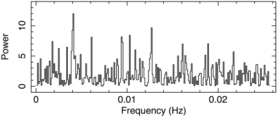
Computing the Rayleigh power for each possible period in order to construct a complete periodogram is orders of magnitude slower than computing the fast Fourier transform, but because there were so few photons, with sometimes so much time between each one, that the Rayleigh statistic was really the only reasonable tool to use to search for a periodic modulation in the arrival times. Naturally, this is what they do with this data set, with these 5063 photon arrival times, testing a lot more frequencies than there are in the Fourier transform—frequencies which are between each independent Fourier frequency. They use the Rayleigh periodogram to compute the power for 20 additional frequencies (so 21 times more than the FFT). This is exactly what allows the second scientist to look in very fine detail at what is happening in the entire spectrum, and especially also in between the independent frequencies. The result is this:

Rayleigh periodogram of event arrival times.
As you can see, we can’t see much from this periodogram. But because whenever they make a Rayleigh periodogram they always see a sharp rise in power at the lowest frequencies, they also always just ignore this, cutting it out of the view and rescaling the y-axis to see the rest of it better, like this:

Cropped and rescaled Rayleigh periodogram shown previous figure.
Lo and behold they discover that there is a peak that clearly stands out of the noise. Excluding the lowest frequency part, the peak stands out of the rest of the periodogram, which just looks like statistical fluctuations similar to those seen in the Fourier transform by the first scientist. The signal is very obvious, right there at a frequency of just over 4E-3 Hz. This is equivalent to a period of just under 250 seconds.
But is it okay to simply ignore part of the periodogram like that, and just focus on what looks interesting? Why is the signal so clear in the Rayleigh periodogram and absent from the Fourier transform? And why in the world does the Rayleigh periodogram have this sharp rise to huge powers at the lowest frequencies? Why doesn’t the Fourier transform have that? Can you really trust that the peak in the Rayleigh periodogram is indeed a signal and not just a fluke, a fluctuation similar to those that are seen at the lowest frequencies but that just happened to appear at a different spot?
As we saw earlier, a major difference between the Fourier transform and the Rayleigh periodogram is that the former is computed on a binned time series, which means it cannot take into account the time of arrival of each detected photon. And this is precisely what the latter does. But there is another major difference between them: the Fourier transform of a binned time series tests only independent frequencies. These are frequencies that correspond to periods that can fit an integer number of times in the time series.
The longest period that can be tested for in a time series lasting T=10000 s can obviously not be longer than 10000 s since we cannot test for periods longer than the duration of the observation. A period of ten thousand seconds is equivalent to a frequency of 1/T or 1E-4 Hz. After that, the time series can be tested for a period of 5000 s that fits two times in the time series, and this corresponds to a frequency of 2/T or 2E-4 Hz. Next, it can be tested for a period of 3333 s that fits exactly three times in the length of the observation and corresponds to a frequency of 3/T or 3E-4 Hz. And so on. So, basically, the only frequencies that can be tested are multiples of 1/T up to 1/2dt, where dt is the timescale of the binning, which in our case was 20 seconds, and hence a maximum frequency of 1/40 or 0.025 Hz.
The Rayleigh periodogram, because it is unbinned and uses the exact times of arrivals of the detected events, has no restrictions on the frequencies it can test and for which it can compute the power. That is, it has no restriction in testing how well a sine curve of that frequency matches the rate at which the events were detected. This is why the periodic signal is clearly detected by the Rayleigh periodogram and not seen in the Fourier transform.
In fact, looking even closer at the periodogram we find that the periodic signal peaks precisely at 247 seconds, corresponding to 40.5/T Hz, which happens to be exactly in between two independent frequencies, those of 40/T and 41/T Hz. This is why it literally slipped between the Fourier transform’s fingers. The Fourier transform in this case is like too coarse a comb, a comb with too much space between its teeth, through which a small knot in your hair can just slip and pass unnoticed. Here is what it looks like when we zoom in around the peak and compare the two periodograms:

Zoom showing comparison between Fast Fourier Transform and Rayleigh periodogram.
The third scientist knows the Fourier transform as well as the Rayleigh periodogram, and understands where the differences between them come from. They have also understood why the Fourier transform does not have the huge rise in power at low frequencies—it only tests independent frequencies, while the Rayleigh periodogram does—it tests frequencies that are not independent and for which the powers are therefore correlated. They know that the reason why the Rayleigh periodogram does this is because it is computed as though it were calculating the power only at independent frequencies even if it isn’t. What needs to be done to avoid this—to correct for this effect—is to modify the Rayleigh statistic to account for the fact that we are testing frequencies that are not independent: frequencies (periods) that do not repeat an integer number of times within the span of the observation.
This is an analytical correction, something that can be calculated exactly. They do that and formulate the modification to the Rayleigh statistic with which they compute the periodogram of these data, the same exact 5063 photon arrival times. What they find is this:

Modified Rayleigh periodogram.
And to be absolutely sure that what they have computed is accurate, they compare the result with the Fourier transform. If the computation is correct, the powers at independent frequencies should match, and there should be no rise of power at low frequencies. Hence, they look closely at the low frequency part of the periodogram and find that they agree very well, exactly as they predicted, and exactly as they should. The comparison looks like this:
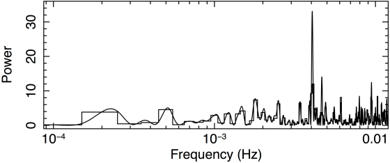
Comparison of Fast Fourier Transform and modified Rayleigh periodogram over entire frequency range.
The first scientist missed detecting the period in the data because they assumed that the Fourier transform was the best they could do in exploring the frequency space of these data, and that information of the independent frequencies was enough to fully characterise the signal when transforming it from intensity as a function of time to power as a function of frequency. The fact is, they most probably would never have known that there was a period in the data, because they would never have looked at these data again.
The second scientist detected the period in the data, but they were forced to arbitrarily cut out a part of the data, simply ignore it, and presume that the height of the peak was the correct power estimate for the periodic signal at 247 seconds. They did this because they had assumed that the Rayleigh statistic, which does not have any restrictions as to the frequencies it can test in a given data set, could be used to compute the power at any frequency, regardless of whether or not it was of an integer number of cycles within the observation duration.
The third scientist detected the periodic signal present in the 5063 arrival times of the detected X-ray photons, but unlike the second scientist, they did not exclude any portions of the data, and got an estimate of the power of the signal from which they could calculate precise and reliable quantities about the signal such as the probability of it having been a statistical fluctuation (1E-9), and the pulsed fraction of the signal, that is, the number of photons right on the sine curve with respect to the total (10%). Both of these, the second scientist would have gotten wrong. Not completely wrong, but wrong nonetheless.
How often does this happen in science? How often does it happen in medical trials? In trials testing a new critical procedure or a new drug? How often does this happen in industry? In testing of a new industrial machine or a new diagnostic technique?
How often does this happen to us in our own life? How often do we infer something, draw a conclusion, make a decision, and act based on assumptions hidden in our psyche so well that we are not even aware of them? Is there a way to overcome this problem?
My personal feeling is that this happens a lot. It is admittedly hard to measure and quantify, but I suppose with enough time and consideration that it could be done, at least for a handful of cases as the one presented here.
About overcoming this fundamental problem that does at first sight appear unsurmountable for the simple fact that we are biased by something we are not aware of being biased by, I think a solution is, by keeping this issue in mind, to not settle for something that can potentially, even hypothetically, be improved upon. In this way, we at least open up the possibility to go on finding more and more suitable methods, more and more accurate estimates, and more and more reliable answers to the questions we seek to answer.

I suspect that there are two distinct phenomena concealed here. One is the limitations of experience and education of any individual scientist. Her ability to analyze any data set will inevitably be limited by education and experience (and possibly less tangible factors like intelligence and personality). This is why science must be a social activity in which experiments and data are constantly replicated by other members of the scientific community. It is one of the factors, for example, behind Popper’s insistence on falsifiability – scientific conclusions can only ever be provisional because there always remains the possibility of another scientist disproving them later. The hope is that if experiments and data analyses are replicated by enough scientists, individual biases and limitations will come out in the wash (as in your example).
A deeper phenomena reflects the extent to which scientists work within an existing paradigm, doing what Kuhn described as “normal science”. In Kuhn’s interpretation, normal science is focused essentially in maintaining the coherence of the paradigm. The core principles of the paradigm become assumptions which are frequently not visible, and when they are must be confirmed. Thus dark energy and dark matter are “invented” to preserve the existing Einsteinian paradigm (rather as aether was invented in the 19th century to preserve the wave theory of light). This can be more insidious in that alternatives and outlier evidence are ignored or reasoned away to preserve the paradigm. The correction to this kind of assumption or prejudice is what Kuhn calls revolutionary science, those moments in which an existing paradigm is overthrown in favour of a new one.
The ultimate solution lies in your final paragraph. We can never know if our science is ultimately correct, although we can know if it “works” (did we get Apollo XI onto the moon or not?). But that becomes less impossible if we see science, like philosophy, less as a body of knowledge than as an activity – something scientists do.
Best
Shaun
LikeLiked by 1 person
Thanks Shaun. Beautifully said.
LikeLike